Betting Math & Statistical Models: EV Calculator & Monte Carlo Tool

Numbers don’t guarantee wins, but they sure beat guessing. If you’ve ever watched someone confidently place a bet based on nothing more than a hunch or because their cousin’s neighbor swears by a certain team, you’ve witnessed the opposite of what actually works in sports betting. Statistical methods aren’t sexy. They don’t come with dramatic stories or gut-feeling heroics. But they do something far more valuable: they reveal patterns hidden in plain sight and help you make decisions that profit over time.

The amateur bettor looks at a team’s win-loss record and thinks they understand everything. The professional bettor sees that same record as barely scratching the surface. What were the circumstances of those wins? Did the team dominate possession but get unlucky with finishing, or did they scrape through with defensive luck that’s bound to regress? Statistics answer these questions, but only if you know which numbers matter and how to interpret them properly.

This isn’t about turning betting into a math exam. You don’t need a statistics degree to apply these methods effectively. What you need is a willingness to look past surface-level results and dig into the underlying performance that actually predicts future outcomes. The bookmakers are already doing this with sophisticated models and teams of analysts. If you’re going up against that infrastructure armed with nothing but recent form and vibes, you’re bringing a calculator to a supercomputer fight.

Monte Carlo Simulations: Calculating Risk of Ruin in 2026

Every successful prediction system starts with expected value, and if you don’t grasp this concept, you’re building on sand. Expected value isn’t complicated despite how intimidating it sounds. It’s simply the average outcome you can expect from a decision if you could repeat it infinite times under identical conditions.

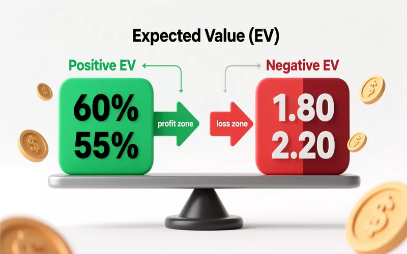
Here’s the thing most bettors miss: you can be right more often than you’re wrong and still lose money. Conversely, you can lose more bets than you win and come out ahead. The magic isn’t in accuracy it’s in the relationship between true probability and the odds you’re getting.

Let’s say a team has a genuine sixty percent chance to win a match. If the bookmaker offers odds of 1.80 on that team, the implied probability is about fifty-six percent. You’ve found positive expected value because the true probability exceeds what the market thinks. Make that bet a hundred times, and you profit. Now flip it: you find a team with a forty percent chance to win, but you’re getting excited because they won their last three games. The bookmaker offers 2.20 odds, implying forty-five percent probability. That’s negative expected value. Win some of those bets? Sure. Profit long-term? Absolutely not.

The math is straightforward. Multiply each possible outcome by its probability, then sum everything up. A ten-dollar bet on something with fifty-five percent true probability paying even money gives you an expected value of one dollar. That doesn’t mean you’ll win exactly one dollar some bets lose, some win. But over sufficient repetitions, that’s your average profit per bet.

Professional bettors obsess over expected value because it’s the only metric that matters across large samples. You’ll see tipsters bragging about sixty-five percent accuracy, but they’re often betting heavy favorites at terrible odds. Their win rate looks impressive while their bankroll bleeds slowly. Meanwhile, the sharp bettor hitting fifty-two percent at positive expected value is quietly banking profit.

The psychological challenge is trusting this over short stretches where variance dominates. You might place twenty positive expected value bets and lose fourteen of them through pure bad luck. Your brain screams that the system is broken. The math whispers to keep going because probability works over sufficient samples, not convenient timeframes.

Probability, Odds, and Converting Between Them

Understanding how probability relates to betting odds is fundamental, yet most bettors operate on feel rather than calculation. Odds are just probability expressed in a format designed to show potential payout, but the relationship between them reveals everything about value.

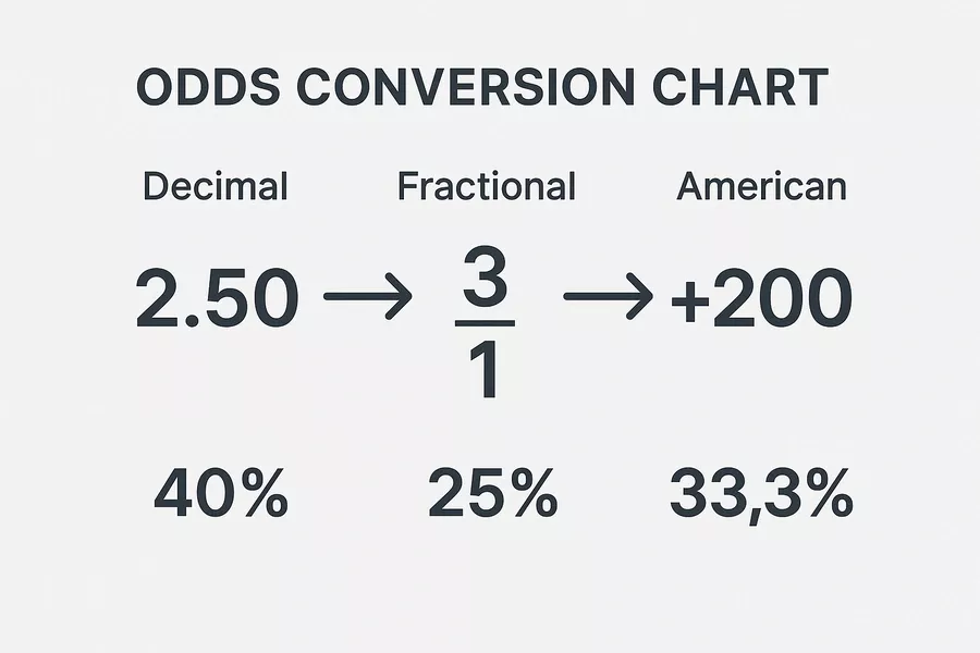
Decimal odds are the cleanest format for this. Take odds of 2.50 and divide one by them: 1 divided by 2.50 equals 0.40, or forty percent implied probability. That’s what the bookmaker thinks is the true chance of that outcome. Fractional odds require slightly more work add the two numbers together and divide the second number by that sum. So 3/1 becomes one divided by four, or twenty-five percent probability.

American odds throw people off initially, but they’re just as logical once you understand the conversion. Positive American odds show profit on a hundred-dollar stake, so +200 means you’d profit two hundred dollars. The conversion formula is 100 divided by (American odds plus 100). For +200, that’s 100 divided by 300, giving you 33.3 percent probability. Negative odds show how much you need to stake to profit one hundred dollars. So -150 means you stake 150 to win 100. The formula flips: negative odds divided by (negative odds plus 100). For -150, that’s 150 divided by 250, or sixty percent.

These conversions matter because they let you instantly spot value. If you’ve analyzed a match and determined the true probability is fifty-five percent, you can quickly calculate that you need odds of at least 1.82 to have positive expected value. Anything below that is a pass regardless of how confident you feel or how much you like the team.

The bookmaker’s margin often called the overround or vig creates the gap you need to overcome. Add up the implied probabilities of all possible outcomes in a market. In a fair market, they’d sum to exactly one hundred percent. Real betting markets sum to 105 or 110 percent because the bookmaker builds in their profit margin. That extra percentage is your cost of doing business. You need to find odds that beat both the true probability and compensate for that margin.

Here’s where most casual bettors fail: they convert the odds, see the implied probability is forty percent, think “that seems about right,” and bet. They never actually calculate the true probability themselves. They’re just confirming the bookmaker’s assessment and paying the margin for the privilege. Sharp bettors do the opposite they determine their own probability first, then shop for odds that exceed what that probability deserves.

Key Metrics That Actually Matter

Sports statistics are endless, but most are descriptive noise that tells you what happened without predicting what happens next. The trick is separating signal from static, focusing on metrics with genuine predictive power while ignoring vanity stats that look impressive but mean nothing.

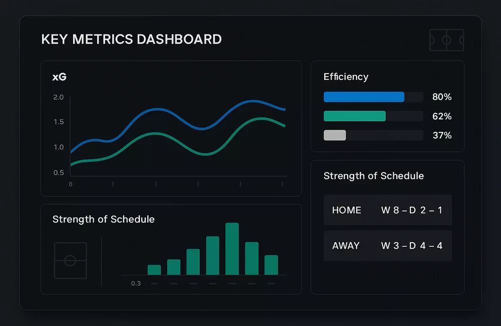
Points per game seems useful until you realize it’s heavily influenced by pace and opposition quality. A team averaging 85 points sounds better than one averaging 78, but what if the first team plays at breakneck speed against weak defenses while the second controls tempo and faces elite competition? Raw scoring tells you nothing without context.

Possession percentage in football might be the most overrated stat in all of sports. Teams can dominate possession and create nothing of value, or they can have thirty percent possession and generate higher quality chances through efficient counter-attacking. What matters isn’t the ball it’s what you do with it when it matters.

Expected goals has revolutionized football analysis precisely because it measures shot quality rather than just counting attempts. A team with fifteen shots sounds dangerous until you see they were all from thirty yards with defenders in the way. Meanwhile, their opponents had five shots, all from inside the six-yard box. Expected goals quantifies this by calculating the historical conversion rate from each shot location and situation. It’s not perfect it can’t account for exceptional finishing ability or goalkeeper quality perfectly but it’s dramatically better than raw shot counts.

Efficiency metrics beat volume stats in almost every sport. In basketball, true shooting percentage accounts for the fact that three-pointers and free throws have different values than two-pointers. A player shooting forty percent from the field sounds mediocre, but if they’re launching threes at high volume and getting to the free-throw line frequently, their true shooting percentage might be excellent. Points per possession measures offensive efficiency better than points per game because it normalizes for pace.

Strength of schedule adjustments turn meaningless stats into useful ones. That team with an amazing defensive record might have played the five worst offenses in the league. Adjust for opponent quality and their defense looks merely average. Conversely, an offense that looks mediocre against tough competition might be quite good. Simple strength of schedule metrics exist publicly, but sophisticated ones that weight recent opponent performance more heavily than early-season games provide better insight.

Home and away splits reveal more than you’d expect. Some teams perform radically different in these situations, and the gap often relates to travel, altitude, crowd impact, or simply psychological factors. In baseball, park factors are massive some ballparks inflate scoring by twenty percent compared to neutral environments. Ignoring these splits means comparing apples to oranges.

Rest and schedule density matters enormously in certain sports. NBA teams on the second night of a back-to-back, especially with travel, perform measurably worse. The fatigue shows up most clearly in second halves and in shooting percentages. NFL teams coming off a bye week have a systematic advantage. Baseball starting pitchers on short rest see velocity and effectiveness decline. These aren’t abstract factors they show up consistently in the data.

The key is building a mental model of which metrics predict future performance versus which just describe past results. Wins and losses are outcomes. Shot quality, efficiency ratings adjusted for opponent, and underlying process metrics predict future wins and losses. Focus your analysis on the latter, use the former only to verify your model is working.

Regression Models and Their Application

Regression analysis sounds intimidating, but it’s just a way to understand relationships between variables and use them to make predictions. At its core, regression asks: when this thing changes, how much does that other thing typically change? Apply that to sports, and you’re modeling how various factors influence outcomes.

Simple linear regression is the starting point. You’re predicting one variable based on another. Maybe you want to predict football match goals based on expected goals from previous matches. Plot the data points, draw the line of best fit, and you’ve got a basic model. The slope tells you the relationship strength how much a one-unit increase in xG predicts for actual goals. The intercept is your baseline. Together, they let you forecast.

The beauty and limitation of simple regression is that sports aren’t simple. Goals don’t depend solely on xG. They’re influenced by opponent defensive quality, weather, motivation, injuries, and countless other factors. This is where multiple regression becomes valuable. You’re predicting one outcome based on multiple input variables simultaneously, accounting for how they interact.

Building a multiple regression model for match outcomes might include variables like home advantage, team efficiency ratings, rest days, historical head-to-head performance, and current form metrics. The model weighs each factor according to its historical predictive power, then outputs a predicted outcome. The sophistication comes in choosing which variables to include and how to prepare them.

Feature engineering creating new variables from raw data often matters more than the regression technique itself. Raw possession percentage might not predict well, but possession in the final third might. Shots on target might be weak, but big chances created could be strong. The art is transforming available data into features that actually correlate with outcomes.

Overfitting is the silent killer of prediction models. You can build a regression model with thirty variables that perfectly “predicts” historical results but fails miserably on new data because it’s essentially memorized noise rather than learned patterns. The model might discover that teams wearing blue shorts on Wednesdays have won historically, then try to apply that meaningless correlation going forward.

The solution is keeping models relatively simple and testing them on out-of-sample data results they haven’t seen during training. Professional modelers split their data, training on eighty percent and testing predictions on the remaining twenty percent. If the model performs well on both sets, you’ve likely captured real patterns rather than random noise.

Logistic regression works better than linear regression for predicting binary outcomes like win-lose. Linear regression assumes your outcome variable can be any number, but match results are discrete. Logistic regression outputs probabilities between zero and one, making it perfect for betting markets where you need to compare your probability assessment to the bookmaker’s implied odds.

The practical application for bettors is that you don’t necessarily need to build these models yourself. Understanding how they work helps you evaluate models others create and recognize their limitations. Many prediction sites use regression models but don’t show their work. Knowing the methodology lets you assess whether their approach is sound or if they’re overfitting data and selling the results as expertise.

Poisson Distribution for Goal Prediction

The Poisson distribution is one of those mathematical tools that sounds academic but proves remarkably practical for betting. It models how often events occur in fixed intervals when those events happen independently at a constant average rate. For goal-based sports like football and hockey, this description fits nearly perfectly.

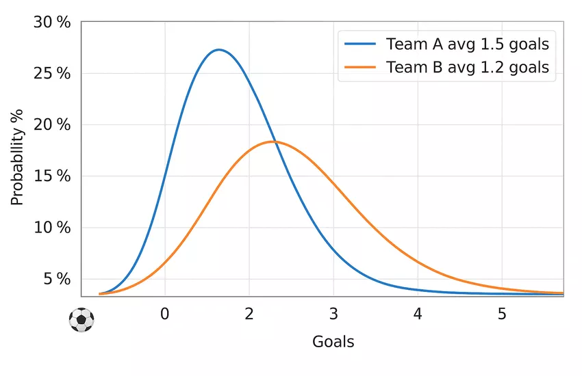
Here’s the logic: if a team averages 1.5 goals per match based on underlying metrics, the Poisson distribution can tell you the probability they score exactly zero goals, one goal, two goals, and so on. Do this for both teams in a match, combine the probabilities, and you can calculate the likelihood of various score lines and outcomes.

The math involves exponentials and factorials, but don’t let that scare you off. Excel and free online calculators handle the computation. What matters is understanding when and why it works. Poisson assumes goals happen independently one goal doesn’t make the next more or less likely. That’s mostly true in football, though not perfectly. Teams that go ahead might park the bus, changing their expected goal rate. Teams behind might open up, increasing goal likelihood at both ends. But as a first approximation, Poisson works surprisingly well.

To use it for match prediction, start with expected goals for each team based on underlying metrics, adjusted for opponent defensive quality. Let’s say Team A averages 1.6 expected goals per match and Team B allows 1.4 expected goals per match against average opponents. Adjust Team A’s figure to 1.5 accounting for facing this specific defense. Run the same calculation for Team B, getting their expected goals when facing Team A’s defense.

Now apply the Poisson distribution to both figures. You get probability distributions for each team’s likely goal total. Combine them to calculate specific score probabilities. The probability Team A wins is the sum of all score line probabilities where they outscore Team B. The probability of a draw is the sum of all equal score lines. You’ve turned expected goals into match outcome probabilities.

Compare your probabilities to the bookmaker’s implied odds. If you calculate a forty-five percent chance Team A wins but the odds imply only forty percent, you’ve found value. That’s positive expected value regardless of whether this specific match ends with Team A winning.

The approach extends beyond match winners. You can calculate over-under probabilities by summing the probabilities of all score lines that total over or under the line. Under 2.5 goals means summing probabilities for 0-0, 1-0, 0-1, 1-1, and 2-0, 0-2. Both teams to score probability comes from one minus the probability of either team failing to score.

Limitations exist. Low-scoring sports like football have more variance than Poisson perfectly captures. Occasionally teams score four or five goals when the model suggested one. But over large samples, Poisson predictions prove more accurate than eyeballing matches or trusting raw form. The model removes bias and emotional attachment, replacing them with probabilistic reasoning grounded in historical patterns.

Advanced versions adjust for factors Poisson doesn’t capture naturally. You might modify expected goals based on motivation levels a team fighting relegation might outperform their underlying metrics. Or you could adjust for tactical matchups a possession-based team facing a compact defense might underperform their typical xG. These adjustments layer human judgment onto mathematical foundations, combining the best of both approaches.

Monte Carlo Simulations and Scenario Analysis

Sometimes you need to explore thousands of possible outcomes to understand probability distributions properly. That’s where Monte Carlo simulations become invaluable. The name comes from the casino, which is fitting these simulations use randomness to model complex systems where analytical solutions are impractical.

The concept is straightforward. You create a model with uncertain variables, assign probability distributions to those variables, then run the simulation thousands of times with randomly sampled values. Each run produces one possible outcome. Aggregate thousands of runs, and patterns emerge that show you the range of likely outcomes and their probabilities.

For sports betting, this becomes powerful when outcomes depend on multiple uncertain variables. Imagine predicting a basketball total. You need to model both teams’ scoring, which depends on pace, efficiency, opponent defense, rest, and randomness. Rather than trying to calculate an exact answer analytically, you simulate ten thousand games using probability distributions for each factor.

Each simulation might randomly select a pace factor from a normal distribution centered on expected pace, then randomly select shooting efficiency from another distribution, factor in defensive adjustments, and output a total score. Run this thousands of times for both teams, and you get distributions of likely total scores. The median becomes your central prediction, but you also see the uncertainty how often scores fall significantly above or below that median.

This visibility into uncertainty matters for bankroll management and bet sizing. A prediction with a tight probability distribution around the expected outcome justifies larger stakes than a prediction with wide variance where you’re less certain. Monte Carlo simulations quantify that certainty, turning vague feelings into numbers you can use.

Building simulations requires some programming or spreadsheet skill, but the barrier is lower than you’d think. Excel has built-in random number functions and tools for running scenarios. You’re essentially creating formulas that represent your model, then copying them thousands of times with different random inputs. Even basic simulations provide insight sophisticated analysis misses.

The real value shows up in complex scenarios where intuition fails. How often does a team win by more than seven points while the total stays under? Your gut can’t answer that accurately. A simulation that models score progressions and variance can. Want to know the probability that both a specific player scores and his team wins? Simulate the game accounting for scoring distributions and individual player involvement.

Professional bettors use Monte Carlo methods to stress-test their bankroll strategies. They simulate seasons worth of bets using their historical win rate and average odds, running thousands of scenarios to see how often they go broke versus how often they double their bankroll. This reveals whether their risk management is sufficient or if they’re courting ruin.

The limitation is that simulations are only as good as your input assumptions. Garbage in, garbage out applies fully. If your probability distributions don’t reflect reality, the simulation produces misleading results. You’re modeling uncertainty, not eliminating it. The simulation shows what happens if your assumptions hold, not whether those assumptions are correct.

Still, even imperfect simulations beat pure guesswork. They force you to explicitly state your assumptions, which alone improves thinking. They reveal how sensitive predictions are to changes in key variables. And they provide probability ranges rather than false precision, keeping you grounded in the reality that sports outcomes contain irreducible uncertainty.

Practical Implementation and Avoiding Common Pitfalls

Theory means nothing without execution. The gap between understanding statistical methods and actually using them profitably is where most bettors fail. Implementation requires discipline, realistic expectations, and awareness of the traps that snag even sophisticated analysis.

Start simple. The biggest mistake is building an elaborate model with twenty variables before you’ve mastered basic probability conversions and expected value calculations. Begin with one sport, one league, and a straightforward approach. Maybe that’s using expected goals and Poisson distributions for football match predictions. Get comfortable with the process, track results over a few hundred bets, then gradually add sophistication.

Your model needs out-of-sample testing or you’re flying blind. Fit your model to historical data, then test predictions on games it hasn’t seen. If accuracy drops dramatically, you’ve overfit. The model memorized historical noise rather than learning predictive patterns. Pull back complexity, remove variables that don’t add consistent value, and test again.

Data quality matters more than model complexity. A simple model using clean, reliable data beats an elaborate model built on garbage. Verify your data sources, check for outliers that seem wrong, and understand what each metric actually measures. Expected goals from one provider might differ from another based on their methodology. Using both interchangeably introduces noise.

Sample size constraints bite harder than you’d expect. That team has a ninety percent win rate at home over their last ten games sounds dominant. But ten games is nothing. The confidence interval around that estimate is massive. They might be genuinely excellent, or they might have gotten lucky repeatedly. You need dozens of matches minimum before trusting rate statistics, more for rare events.

Avoid the narrative trap where you retrofit statistics to support what you already believe. You want Team A to win, so you emphasize their expected goals while downplaying opponent adjustments. This confirmation bias destroys the value of statistical analysis. The numbers should inform your opinion, not validate it. When statistics contradict your intuition, that’s exactly when they’re most valuable.

Regression to the mean is everywhere in sports, yet bettors constantly ignore it. That striker scored in seven straight matches, so you’re betting anytime scorer. Except his underlying metrics suggest he’s running hot his shot quality doesn’t justify the streak. Regression is coming. That defense hasn’t conceded in five games, but their xG against is mediocre. They’ve gotten lucky with finishing and variance. Don’t extrapolate extremes.

Even with the best math, you must perform a thorough team performance analysis for betting to account for injuries and lineups.

Markets move for reasons. If your model identifies huge value but the line is moving against you, pause before betting. Maybe injury news just broke that your model hasn’t incorporated. Maybe there’s information you’re missing. Sometimes you’ve genuinely found value the market hasn’t recognized yet, but often there’s a reason for the discrepancy. Do additional research before assuming you’re smarter than the collective wisdom.

Bankroll management integrates with statistical methods, not stands apart from them. Your statistical analysis provides win probabilities and expected value. Those feed into optimal bet sizing formulas like Kelly Criterion, which recommends stake sizes based on edge and confidence. Never bet a fixed amount regardless of perceived edge that’s leaving money on the table with strong bets and risking too much on marginal ones.

Track not just wins and losses but the process. Did your predicted probability match reality over sufficient samples? If you predicted sixty percent win probability on twenty bets, you’d expect roughly twelve wins. Getting eight doesn’t necessarily mean your model is broken variance explains that. But if over two hundred bets at sixty percent you’re only hitting fifty percent, your calibration is off. The model systematically overrates winning chances.

Continuous refinement never stops. Last season’s model might need adjustments for rule changes, tactical evolutions, or shifts in how bookmakers set lines. Stay current with your sport. Follow tactical analysts and sharp bettors to understand how the game is changing. Update your variables and weights as new patterns emerge.

The unsexy truth about statistical betting is that it’s boring. There’s no drama, no hot takes, no swashbuckling hero calls. You run your model, it identifies value, you bet, you move on. Most bets lose or win by normal variance, not because you’re brilliant or stupid. Over thousands of bets, small edges compound into consistent profit. That’s the entire game. Embrace the boredom, trust the math, and let probability work over sufficient samples.

Always look for a bookmaker with license to ensure your data-driven profits are secure.